AMIT 135: Lesson 3 Particle Size Distribution – Mining Mill Operator Training

Contents

Objectives

After completing this lesson students should be able to:

Demonstrate understanding of various method involved in measuring particle size.
Explain the importance of particle size analysis and its application.
Differentiate between the different models used for predicting particle size.
Explain the different convention followed in measuring particle size.

Reading & Lecture

Mineral Particle Sizes

Particles within a given process stream vary in size and shape.
Quantifying the amount of material within a given size fraction is often important for design and operational considerations.
Particles that are either spherical or cubical are relatively easy to characterize.
However, the majority of particles are often neither of these two shape types.
Particle size characterization can be determined by:
- Microscopic Analysis
- Sieving
- Sedimentation (Stokes Diameter)
- Optical (Laser deflection or reflection)

Mean Particle Sizes

The mean particle size of a distribution is typically measured by either the arithmetic or geometric mean of the maximum (dmax) and minimum (dmin) particle sizes.
The arithmetic mean is most accurate for symmetric particles such as spheres or cubes.
$d{am} = \frac{d{max} + d{min}}{2}$
The geometric mean is typically preferred when segregation of the particles into various fraction were achieved by passing particles through an opening having a given shape and area, e.g., screening.
$d{gm} = (dmax * dmin)^{\frac{1}{2}}) = (d{1}d{2}d{3}...d{n})^{\frac{1}{N}}$ N = number of particles or size fractions

Particle Size Analysis

Sieve Opening Size (mm)		Mean Particle Size (mm)	Weight (#)	Cumul. % Retained	Cumul. % Finer
Passed	Retained
(1*2^.5)	1.0	1.19	5.0	5.0	100.0
1.0	0.6	0.77	10.0	15.0	95.0
0.6	0.3	0.42	25.0	40.0	85.0
0.3	0.15	0.21	40.0	80.0	60.0
0.15	pan	0.01	20.0	100.0	20.0
Total			100.00

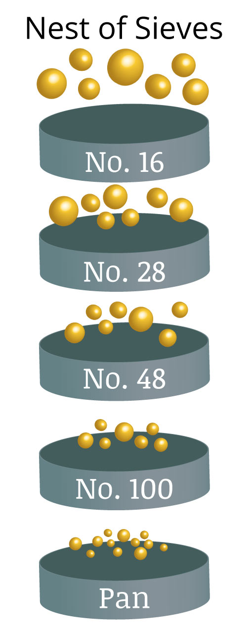
Nest of Sieves — Diagram of a nest of sieves.

The top size was estimated to be the square root of two times the top sieve size or 1.4mm.
There is 5% retained on the 1mm screen.
If the total feed was directed to the 0.3mm screen, 40% of the feed would be retained on the screen.
95% of the feed is finer than 1mm and 20% is finer than 0.15mm.
The mean size of the material passing the 0.15mm screen can be estimated assuming the bottom size is 1 micron.

Particle Sizes Distribution Models

There is a common need to determine the amount of material in the feed at a given particle size.
The desired particle size may not have been included in the original particle size analysis.
The two common models used include:

Gates-Gaudin-Schuhmann Model (GGS)
Rosin-Rammler Model (RR)

The RR model is typically satisfactory for coarse distributions.
The GGS model is generally considered more precise for fine particle size distributions.
It may be needed to perform model fits over more than 2 particle size rangers.

Gates-Gaudin-Schumann Model

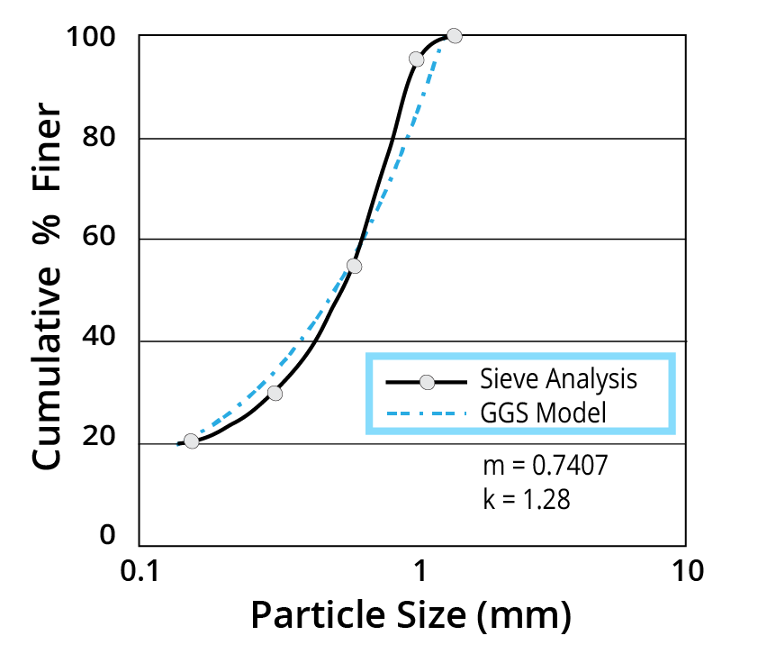
The GGS model predicts the cumulative percent passing distribution:

$Y = 100(\tfrac{x}{k})^{m}$

Y= cumulative percent passing

x= particle size

k= size parameter

m =distribution parameter

The values of k and m can be determined by linear regression:

log y = m log x + k

Rosin-Rammler Model (RR)

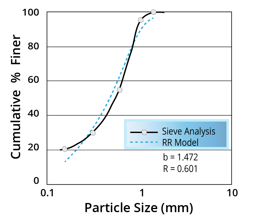
The Rosin-Rammler model is typically used to predict the % retained.
The modified equation to predict the % finer is: $Y = 100 - 100exp \left [ -\left ( \frac{x}{R} \right )^{b} \right ]$

R= size parameter

b= distribution parameter

There is special graph paper available to help determine the correct values of R and b over any size range.

Volume Mean Diameter

The mean particle size by volume is important when dealing with topics such as material transport, storage and hindered particle settling velocities.

The volume mean diameter, $d_{3}^{v}$ , can be quantified by:

$d_v = \left (\frac{\sum_{i=1}{M_i}}{\sum_{i=1}\frac{M_i}{d^3}} \right )^\frac{1}{3} = \left ( \frac{1}{\sum_{i=1}\frac{M_i}{d^3}} \right )^\frac{1}{3}$

Where $M_{i}$ is the mass within size fraction i.

Mean Size Fraction Diameter (mm)	d_p³	Mass, M_i (%)	M_i/d³
0.8	0.512	10	19.53
0.6	0.216	40	185.19
0.3	0.027	30	1111.11
0.125	0.002	20	10000
Total		100	11315.83

$d_v = \left ( \frac{100}{11315.83} \right )^\frac{1}{3} = 0.206mm$

Surface Mean Diameter

The surface mean diameter is important when considering surface coatings with chemicals, particle agglomeration and dewatering.
The volume mean diameter, d_s, can be quantified by: $d_{s} = \left ( \frac{particle mass per diameter}{particle mass per volume} \right )^{\frac{1}{2}} = \left ( \frac{\Sigma_{i-1} \frac{M_{i}}{d_{i}}}{\Sigma_{i-1} \frac{M_{i}}{d^{3}}} \right )^{\frac{1}{2}}$
where M_i is the mass within the size fraction i.

Mean Size Fraction Diameter (mm)	$\dpi{200} d_{3}^{p}$	Mass, M_i (%)	$\dpi{200} \frac{M_{i}}{d_{3}^{i}}$	$\dpi{200} \frac{M_i}{d_i}$
0.8	0.512	10	20	13
0.6	0.216	40	185	67
0.3	0.027	30	1111	100
0.125	0.002	20	10000	160
Total		100	11315	340

$d_{s} = \left ( \frac{340}{11316} \right )^{\frac{1}{2}} = 0.173$

Save