Contents
Objectives
Upon completing this lesson students should be able to:
- Explain the method used to assess the performance of separators.
- Illustrate partition analysis for comminution circuit.
- Analyze different types of partition curves.
- Explain the methods to access separation efficiency from partition curve.
Reading & Lecture
Partition Analysis
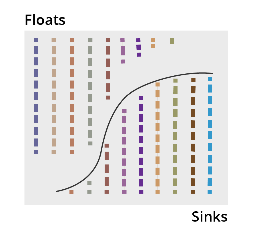
- One of the most insightful methods for quantifying the performance of separators is a “partition analysis’.
- This detailed assessment is commonly performed using a “partition curve’.
- Partition curves show the probability of a particular particle having a given characteristics reporting to a given product stream.
- Can be achieved for any separation: particle size, density, magnetics, floatability, etc.
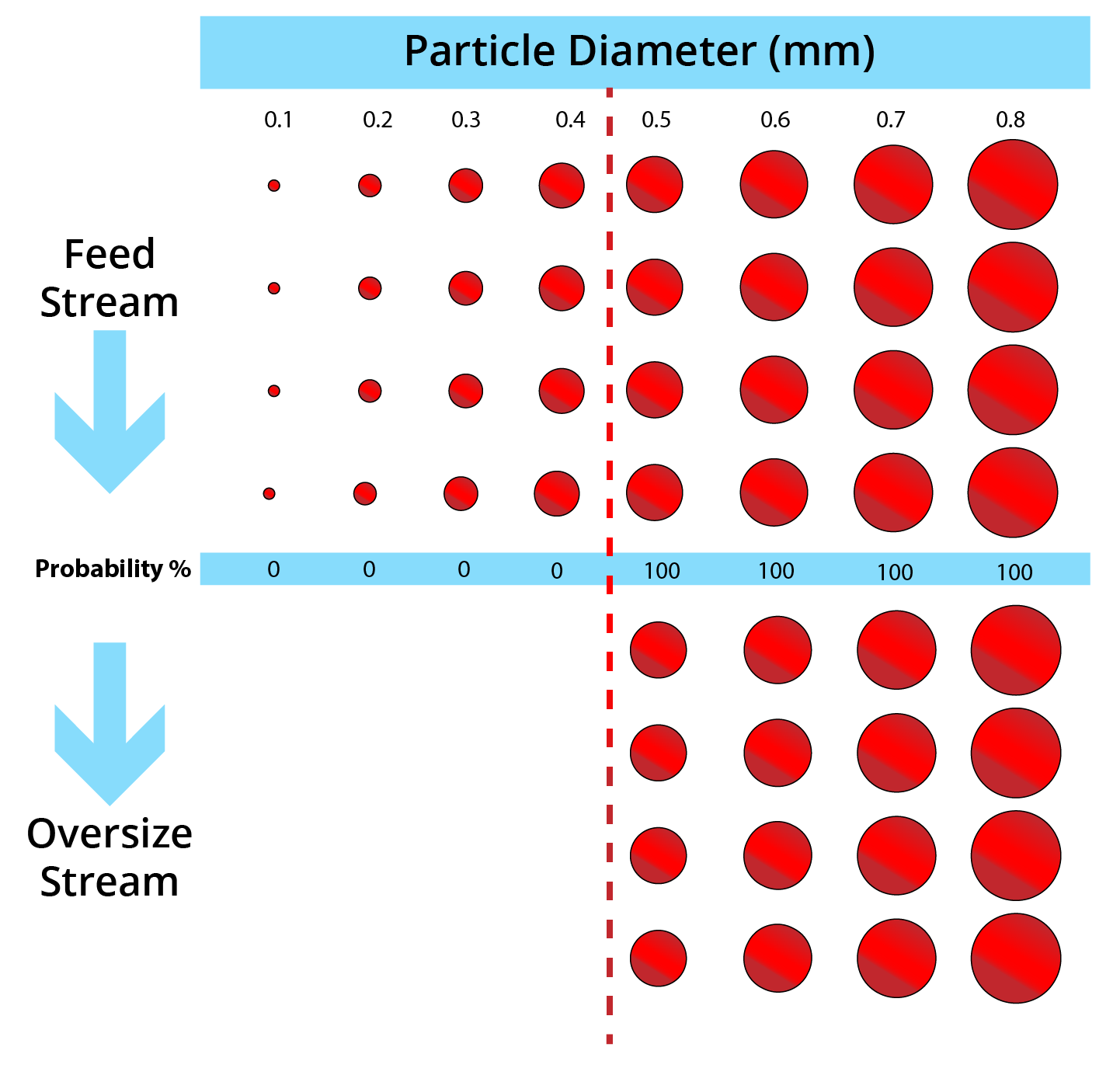
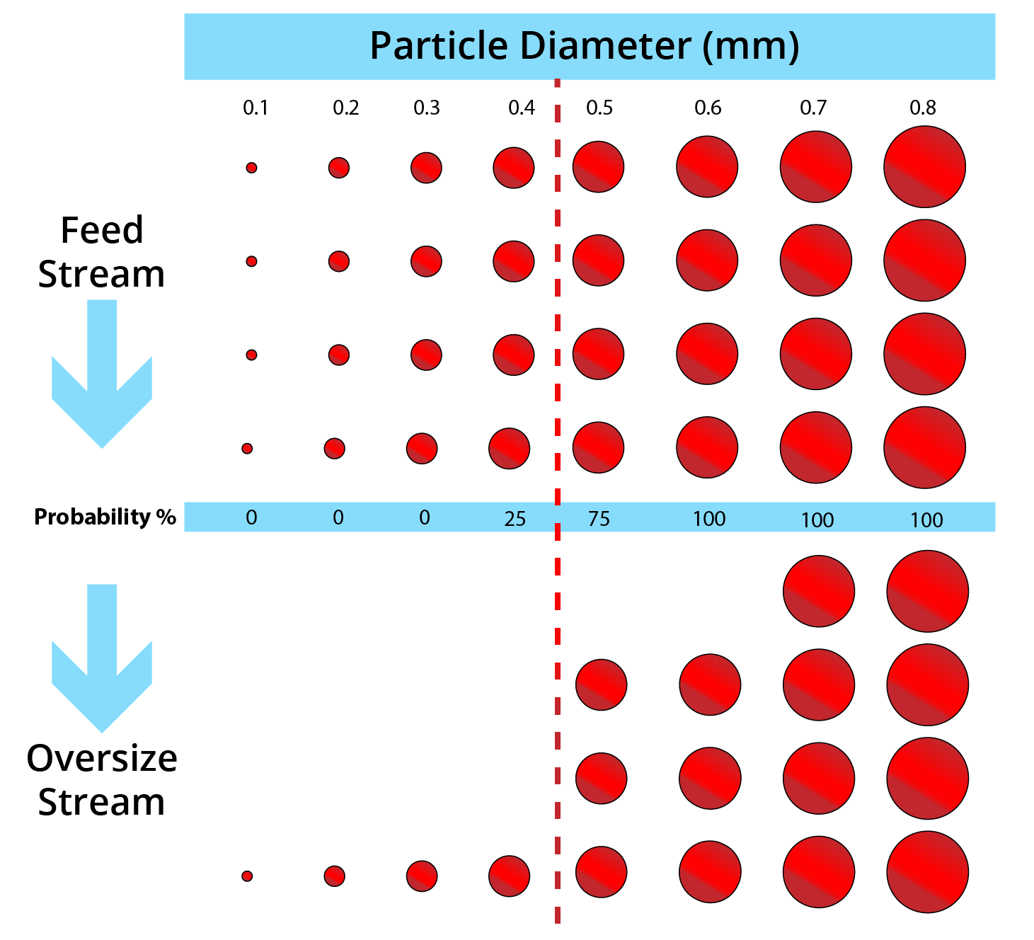
- To explain partition curves, let’s take a look at a “perfect’ particle size separation at 0.45 mm.
- As shown, 100% of particles > 0.45 mm in each in each size class in the feed report to oversize.
[image: (135-4-2)]
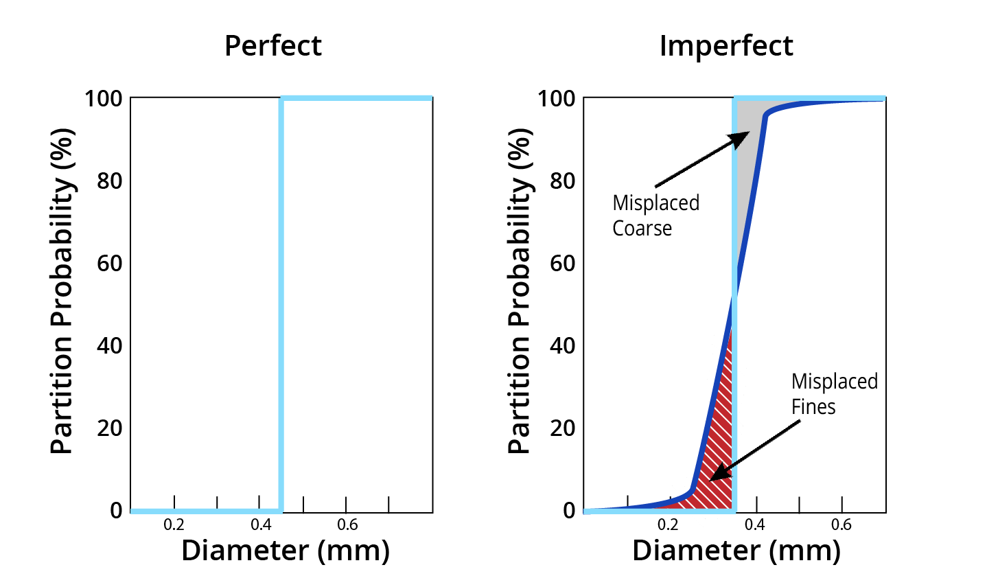
- If the separation is less than perfect, then particles can be “misplaced’ to the wrong streams.
- This includes:
- Misplacement of coarser particles to undersize
- Misplacement of finer particles to oversize

[image: (135-4-3)]
[image: (135-4-4)]
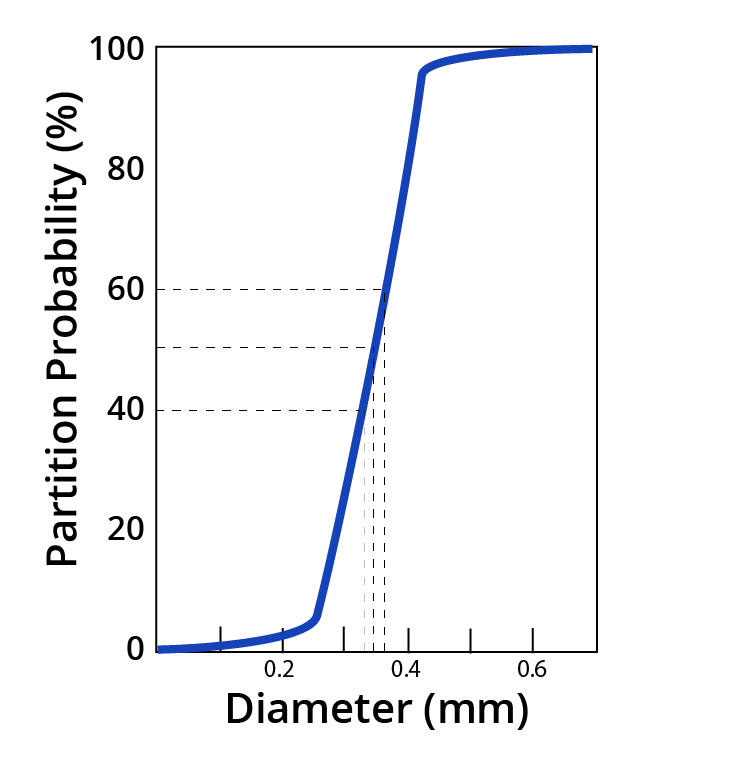
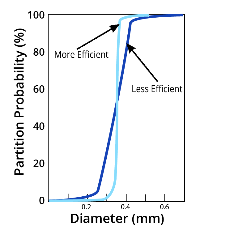
- If ideal, curve runs parallel to abscissa at the “cutsize’.
- More deviation from axis means more misplaced material.
- Shape is characteristic of separator type and operation.
- Cut — Point
= D50
= 0.45 mm
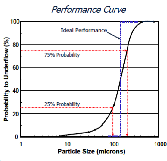
- Ecart Probability (Ep)
= [D75-D25]/2
=(0.5-0.4)/2=0.05 mmImperfection (I)
=EP/D50
=0.05/2 = 0.025
[135-4-5]
- Curve shape is an inherent characteristic of the type of separator employed.
- Commonly reported values for imperfection range from 0.005 to more than 0.50.
- Depends on:
- Type of equipment (e.g., screens, cyclones hydraulic sizers, etc)
- Characteristics of feed material (e.g., particle size, shape, density, etc.)
- Production demands (feed rate, water quality, etc.)
[image: (135-4-6)]
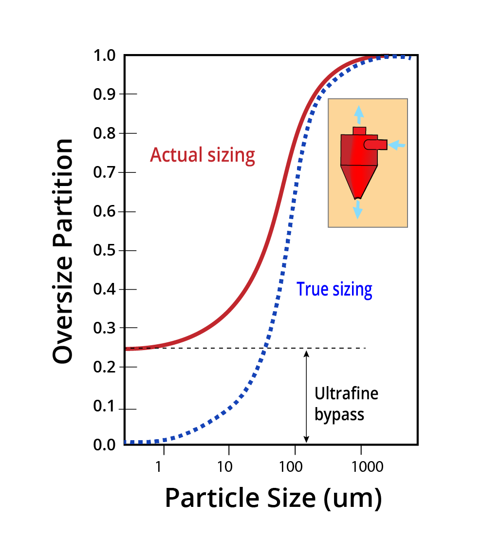
- Another important issue is “bypass’.
- Bypass can occur to both oversize and undersize.
- Oversize bypass is not unusual for screens
- Undersize bypass very common for classifiers.
[image: 135-4-7)]
- Bypass is the misplacement of fines via entrainment into the oversize product.
- Quantified by zero-size offset on the partition curve.
- Can sometimes >30 °/o for fine sizing applications.
- Bypass typically has a large adverse downstream impact.
- Classifiers are often used in multiple stages to reduce bypass (i.e., retreat oversize).
Acceptable Curves:
- Type 1- Ideal Symmetrical
- represents perfect processes (e.g., laboratory sieve data)
- Type 2 – Efficient Symmetrical
- OK for efficient units (e.g., well designed/operated screen)
- Type 3 – Inefficient Symmetrical
- OK for less efficient units (e.g., fine hydraulic classifiers)

[image: (135-4-9)]
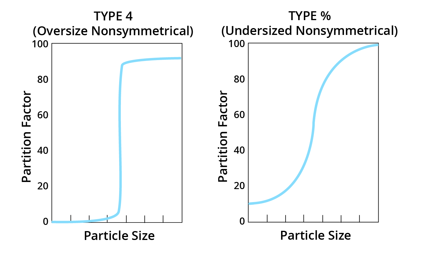
Undesirable Curves:
- Type 4- Oversize Nonsymmetrical
- shows loss of coarse to undersize (e.g., holes in screens)
- Type 5 – Undersize Nonsymmetrical
- shows loss of fines to oversize (e.g., overloaded screen)
[image: (135-4-10)]
Inherent unit characteristic, poor circuit design, excessive rates, mechanical failure, poor operating practices, others …
Step 1- Collect Samples
- Collect representative samples of the feed, oversize and undersize streams.
- Make sure that all streams have been taken into account.
Step 2 – Perform Size Analysis
- Perform a laboratory particle size analysis on each sample.
- Assess data to make sure that it is reliable (discussed later).
| Size Class (Mesh) | Mean Size (mm) | Feed Mass (%) | U/S (%) | O/S (%) |
|---|---|---|---|---|
| +10 | 2.404 | 4.02 | 0.00 | 7.85 |
| 10x20 | 1.202 | 4.68 | 0.12 | 11.78 |
| 20x28 | 0.714 | 13.41 | 1.88 | 26.50 |
| 28x35 | 0.505 | 11.20 | 3.82 | 18.10 |
| 35x48 | 0.357 | 5.03 | 3.53 | 7.20 |
| 48x65 | 0.252 | 10.86 | 11.52 | 10.08 |
| 65x100 | 0.178 | 12.50 | 16.29 | 7.19 |
| 100x150 | 0.126 | 14.27 | 20.96 | 5.72 |
| 150x200 | 0.089 | 8.40 | 15.30 | 2.28 |
| 200x325 | 0.058 | 10.25 | 17.52 | 2.16 |
| -325 | 0.030 | 5.39 | 9.06 | 1.14 |
| 100.0 | 100.0 | 100.0 |
Step 3 – Conduct Calculations
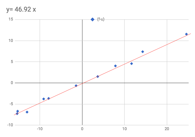
- Plot (u-f) versus (u-o).
Data should form a line passing through zero . - Line slope is the fraction of feed tonnage that reports to oversize.
- You may disregard unreliable points that do not appear to fall along the line.
| Size Class (Mesh) | Mean Size (mm) | Feed Mass (%) | U/S (%) | O/S (%) | X-axis (u-o) | Y-axis (u-f) |
|---|---|---|---|---|---|---|
| +10 | 2.404 | 4.02 | 0.00 | 7.85 | -7.85 | -4.02 |
| 10x20 | 1.202 | 4.68 | 0.12 | 11.78 | -11.66 | -4.56 |
| 20x28 | 0.714 | 13.41 | 1.88 | 26.50 | -24.62 | -11.53 |
| 28x35 | 0.505 | 11.20 | 3.82 | 18.10 | -14.28 | -7.38 |
| 35x48 | 0.357 | 5.03 | 3.53 | 7.20 | -3.67 | -1.50 |
| 48x65 | 0.252 | 10.86 | 11.52 | 10.08 | 1.44 | 0.66 |
| 65x100 | 0.178 | 12.50 | 16.29 | 7.19 | 9.1 | 3.79 |
| 100x150 | 0.126 | 14.27 | 20.96 | 5.72 | 15.24 | 6.6 |
| 150x200 | 0.089 | 8.40 | 15.30 | 2.28 | 13.02 | 6.90 |
| 200x325 | 0.058 | 10.25 | 17.52 | 2.16 | 15.36 | 7.27 |
| -325 | 0.030 | 5.39 | 9.06 | 1.14 | 7.92 | 3.67 |
| 100.0 | 100.0 | 100.0 |
[image: (135-4-11)]
Step 4 – Construct Partition Curve
- Calculate oversize partition for each size class using [(u-f)o]/[(u o)f].
- Plot mean size versus partition factor .
- Compute performance indicators (cutsize, imperfection, bypass, etc.).
| Mean Size (mm) | Feed Mass (%) | U/S (%) | O/S (%) | Y-axis (u-f) | X-axis (u-o) | Percent Feed Weight U/S | Percent Feed Weight O/S | Reconstituted Feed Weight | Partition Number |
|---|---|---|---|---|---|---|---|---|---|
| 2.404 | 4.02 | 0.00 | 7.85 | 4.02 | 7.85 | 0.00 | 3.68 | 3.68 | 100.00 |
| 1.202 | 4.68 | 0.12 | 11.78 | 4.56 | 11.66 | 0.06 | 5.53 | 5.59 | 98.86 |
| 0.714 | 13.41 | 1.88 | 26.50 | 11.53 | 24.62 | 1.00 | 12.43 | 13.43 | 92.57 |
| 0.505 | 11.20 | 3.82 | 18.10 | 7.38 | 14.28 | 2.03 | 8.49 | 10.52 | 80.73 |
| 0.357 | 5.03 | 3.53 | 7.20 | 1.50 | 3.67 | 1.87 | 3.38 | 5.25 | 64.32 |
| 0.252 | 10.86 | 11.52 | 10.08 | -0.66 | -1.44 | 6.11 | 4.73 | 10.84 | 43.61 |
| 0.178 | 12.50 | 16.29 | 7.19 | -3.79 | -9.1 | 8.65 | 3.37 | 12.02 | 28.07 |
| 0.126 | 14.27 | 20.96 | 5.72 | -6.6 | -15.24 | 11.13 | 2.68 | 13.81 | 19.43 |
| 0.089 | 8.40 | 15.30 | 2.28 | -6.90 | -13.02 | 8.12 | 1.07 | 9.19 | 11.64 |
| 0.058 | 10.25 | 17.52 | 2.16 | -7.27 | -15.36 | 9.30 | 1.01 | 10.31 | 9.83 |
| 0.030 | 5.39 | 9.06 | 1.14 | -3.67 | -7.92 | 4.81 | 0.53 | 5.34 | 10.01 |
| 100.0 | 100.0 | 100.0 | 53.08 | 46.92 | 100.00 |
Yield to Oversize Stream – 46.92%
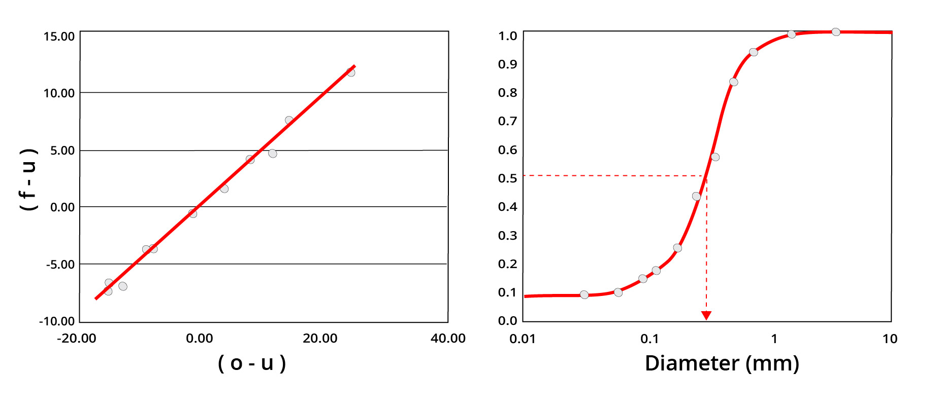
Slope in first plot shows that 46 .9% of feed reported to oversize. Partition curve shows 0.30 mm cutsize, no oversize bypass and 9% undersize bypass. [image: (135-4-12)]
Partition Curve Observations
- The partition curve completed for a particle size separation utilized the weight distribution of all process streams including the feed stream.
- Depending on the breakage characteristics of the material and the location of the sample points, particle breakage could occur which affects the component balance around the process.
- As such, it is sometimes preferred to use component assays (e.g., solid concentration or assays such as iron content) and the two-product equation to determine mass yield.
- Using the mass yield, the feed is then reconstituted to determine the partition numbers.
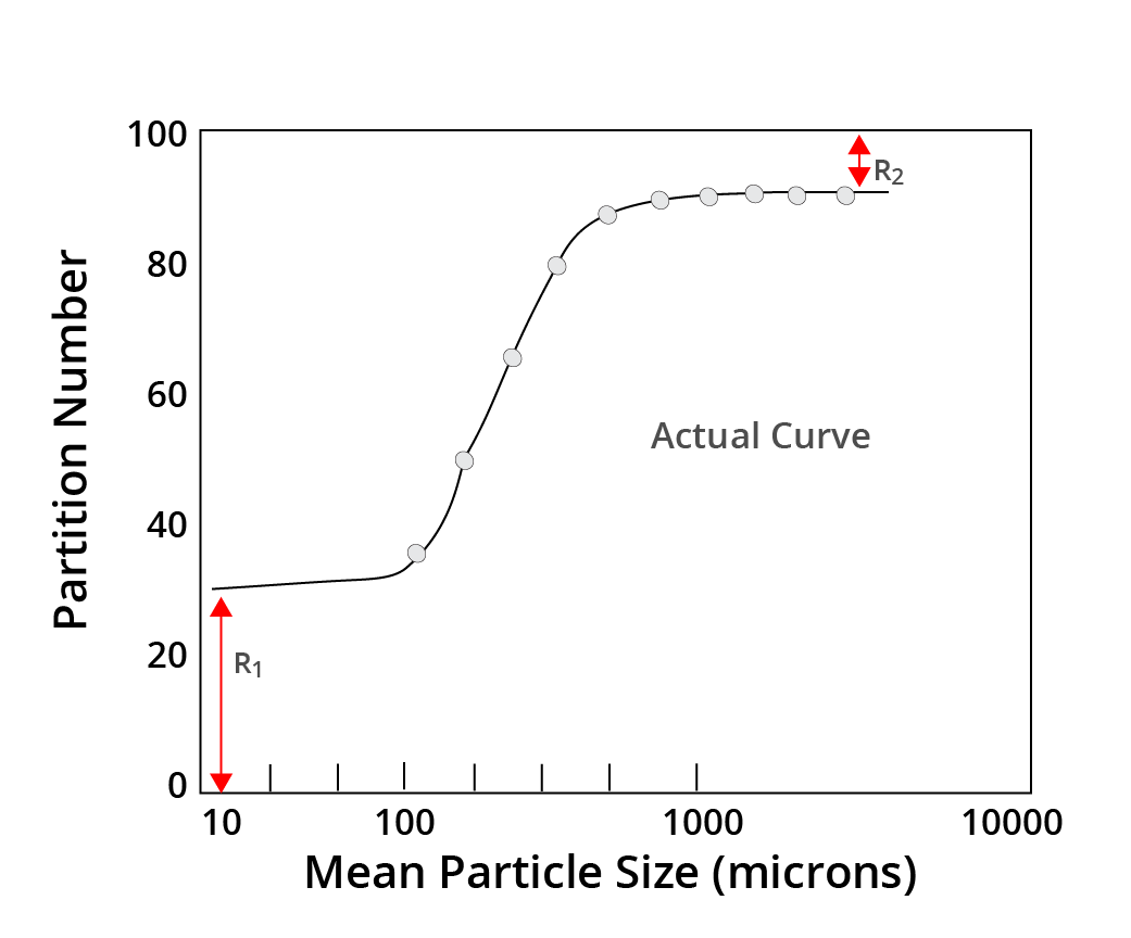
Corrected Partition Number
The equation for determining the corrected Partition Number is:
| (5-10) (5-10) |
Y’ is the corrected partition number, Y the actual partition number, R1 , the fractional amount of ultrafines by-passing to the underflow stream and R2 , the fractional amount of coarsest particles by-passing to the flow stream.
- The by-pass of coarse material to the overflow stream is rare but may occur due to a worn vortex finder.
- R2 =0 can be assumed in most cases.
Separation Efficiency
Separation efficiency should always be measured from the corrected partition numbers.
- Bypassed particles were not subjected to the separation forces .
For particle size separations, the imperfection value (I) is the preferred measurement:
d75, d50 , and d25= the particle size having 75 %, 50% and 25% probabilities, respectively, of reporting to the underflow stream.
[image: (135-4-14)]
Separation Performance Projection
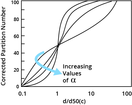
- Many equations are available that model typical performance curves associated with
- Lynch and Rao found that the Reduces Efficiency curve can be modeled by the following expression:
X= d/d 50(c)
α = the curve slope and the value is indicative of the classification efficiency.
- The Lynch model can be used to predict the performance of a classifying cyclones.
Example: Performance Prediction
Given a feed particle size distribution and an alpha value of 2.5, predict the performance of a cyclone. The amount of ultrafine by-pass is assumed to be 20% by weight.
| 1 | 2 | 3 | 4=Eq.[5-10] | 5=Eq.[5-10] | 6=2*5 | 7=6/(∑6) |
|---|---|---|---|---|---|---|
| Mean Particle Size (microns) | Weight (%) | d/d50(c) | Corrected Partition Number | Actual Partition Number | Underflow Weight (%) | Normalized Underflow Weight (% |
| 1200 | 2.40 | 12 | 1.00 | 1.00 | 2.40 | 3.90 |
| 850 | 7.50 | 8.5 | 1.00 | 1.00 | 7.50 | 12.18 |
| 600 | 8.90 | 6 | 1.00 | 1.00 | 8.90 | 14.45 |
| 425 | 6.40 | 4.25 | 1.00 | 1.00 | 6.40 | 10.39 |
| 300 | 6.90 | 3 | 1.00 | 1.00 | 6.89 | 11.19 |
| 212 | 4.30 | 2.12 | 0.97 | 0.97 | 4.19 | 6.80 |
| 150 | 4.50 | 1.5 | 0.82 | 0.86 | 3.86 | 6.28 |
| 106 | 4.00 | 1.06 | 0.55 | 0.64 | 2.55 | 4.14 |
| 75 | 3.40 | 0.75 | 0.31 | 0.45 | 1.52 | 2.46 |
| 53 | 51.70 | 0.53 | 0.17 | 0.34 | 17.36 | 28.20 |
| Total | 100.00 | 61.57 | 100.00 |
Mass Yield to Underflow = 61.57%
Summary
- “Partition factor” represents the probability that a given particle size in the feed stream will report to the oversize product.
- “Partition analysis” makes it possible to determine key performance indicators.
- Cutsize (D50)
- Imperfection (I)
- Bypass
- Plant personnel should monitor and strive to maintain sizing “efficiencies ” since this greatly impacts other plant operations.