Contents
Reading
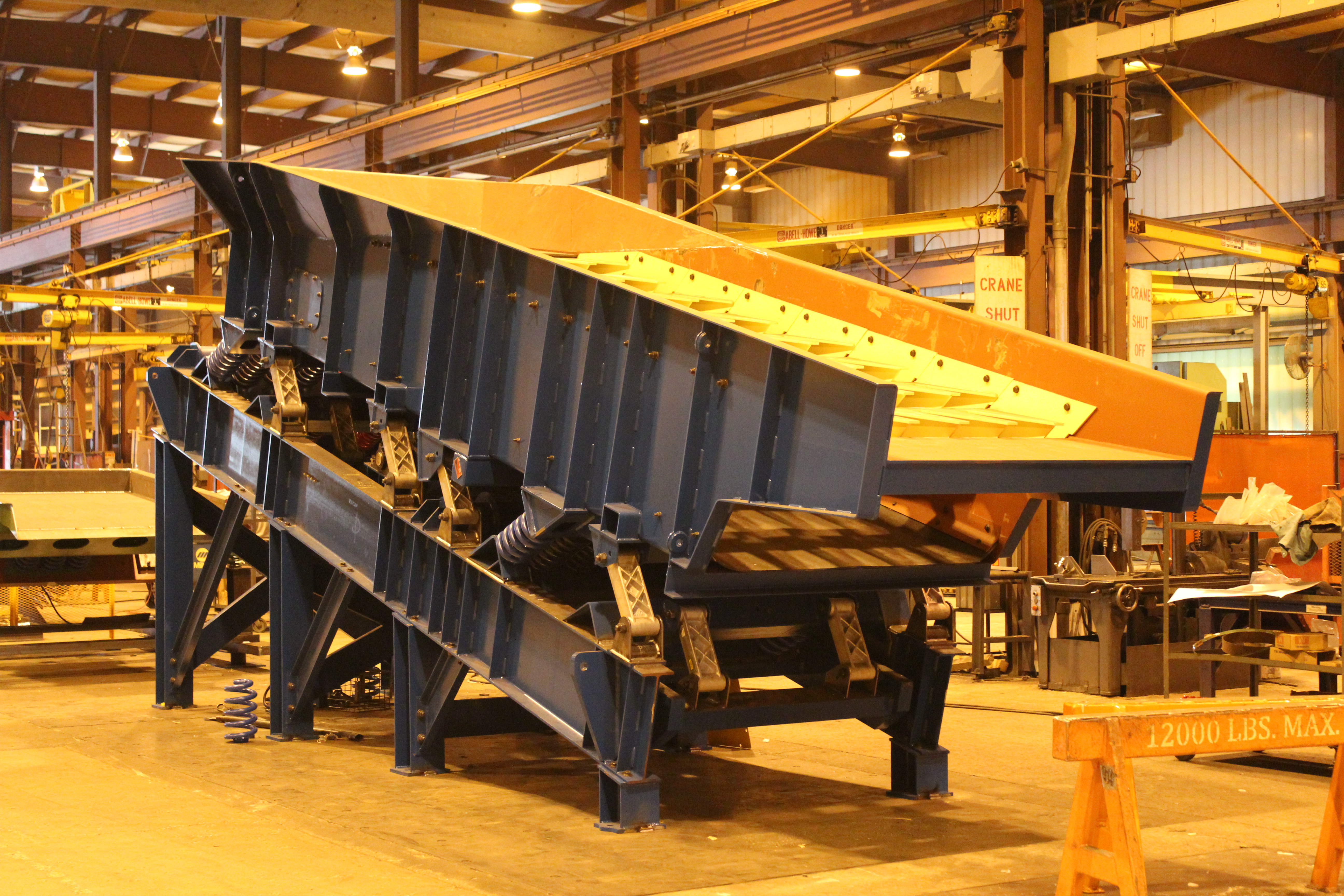
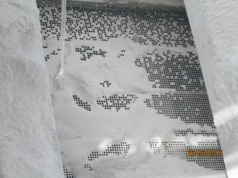
Industrial Screens
- A 20 ° inclined screen is typically used for pre screening and sizing applications.
- Decreasing the inclination slows the movement across the table thereby decreasing capacity but improving efficiency.
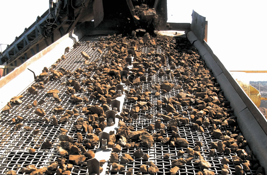
- Above 12 mm, dry screening is preferred.
- Below 12 mm, wet screening using a low-pressure water spray is preferred with a water flow rate of 0.8- 1.4 m3/t/h.
- Actual water requirements dependent on application.
[image 145-1-1a]
![[image 145-1-1a]](https://3t10bc3i56x0ua6sa22vcgim-wpengine.netdna-ssl.com/wp-content/uploads/2015/05/IMG_1421.jpg)
[image 145-1-1b]
![[image 145-1-1b]](https://www.eurobelt.eu/img/accessories/screens/big/pletene_sita_big.jpg)
Screening Fundamentals
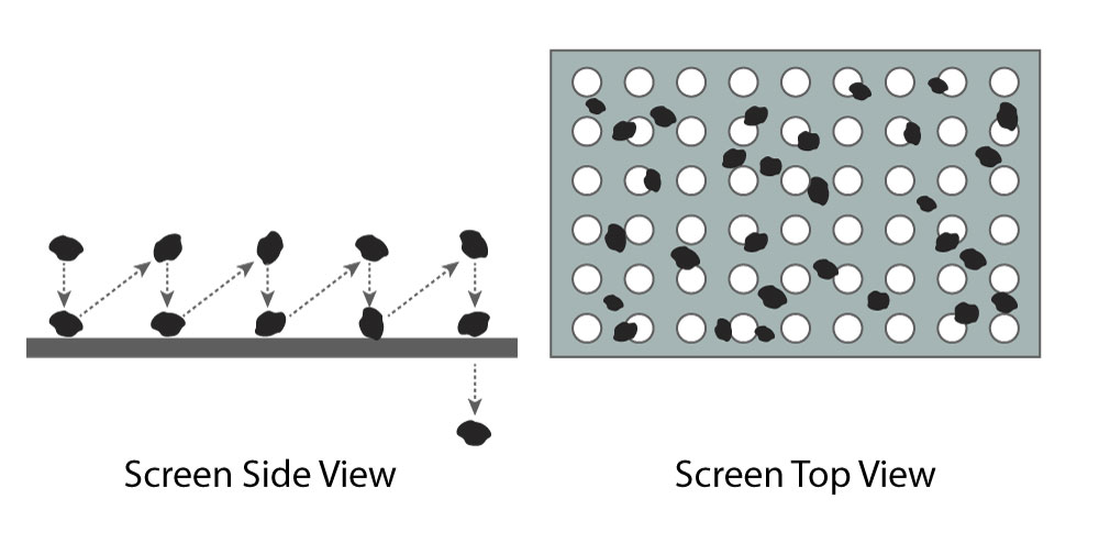
In screening, two basic processes are taking place.
- Stratification -The process whereby the large particles rise to the top of the vibrating material bed while the small particles shift through the voids and form the bottom of the bed.
- Probability of Separation – The process of particles reporting to the screen apertures or openings and passing through if the particle size is less than the aperture
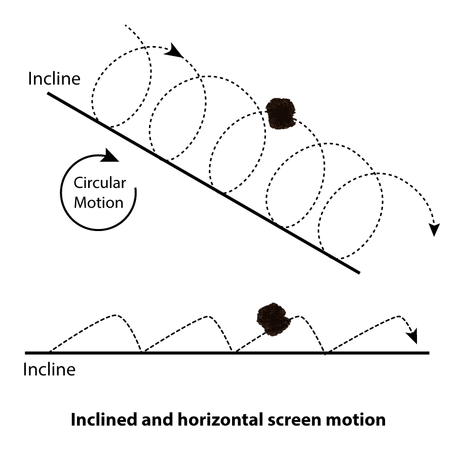
Screen Motion
The processes of particle stratification and probability are caused by the vibration of the screen.
On inclined screens, the vibration is caused by a circular motion in a vertical plane of 1/8 to 1/2- inch amplitude at 700 to 1000 cycles/min. The vibration lifts the particles up, thereby, causing stratification. The incline will cascade the particles down the slope and introduce the probability of particle passage through the screen.
Horizontal screens, which are used only when height restrictions prohibit inclined screens, transfer the material using a straight line motion at an angle of approximately 45 degrees to the horizontal. This motion lifts the particles up from the screen surface and moves the particles toward the discharge end.
Screen Feed Rate Factors
Rule of thumb :
- For particles weighing 100 lbs/ft3 or greater, the bed depth at discharge should never be greater than 4 times the aperture size in the screen.
- For particles less than 100 lbs/ft3, the bed depth is limited to 3 times the opening size.
Other factors controlling stratification include:
- Material travel rate (length/time) is a function of:
- material specifications;
- screening media specifications;
- depth of bed;
- stroke characteristics;
- slope of screen.
- Stroke characteristics
- amplitude;
- direction of rotation;
- type of motion;
- frequency.
- Surface moisture – high surface moisture hinders stratification.
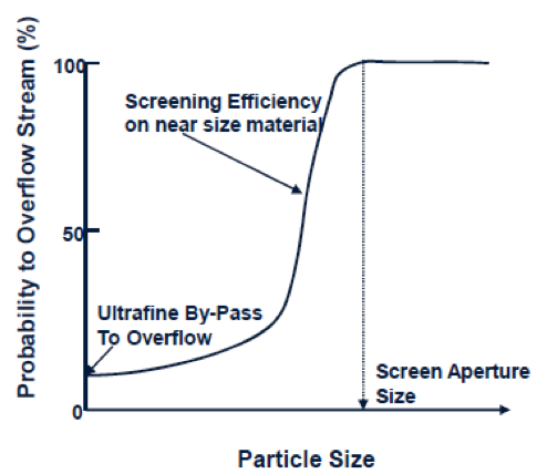
Screening Probability
Upon stratification, the particles having a size less than the smaller screen aperture pass through the screen to the underflow.
Obviously, Particles having a size significantly smaller than the aperture size pass through easily.
However, the probability of P of a particle passing through the screen in one trial decreases as the particle size approaches the aperture size, i.e,
a = screen opening size;
x = particle diameter
b = diameter of wire
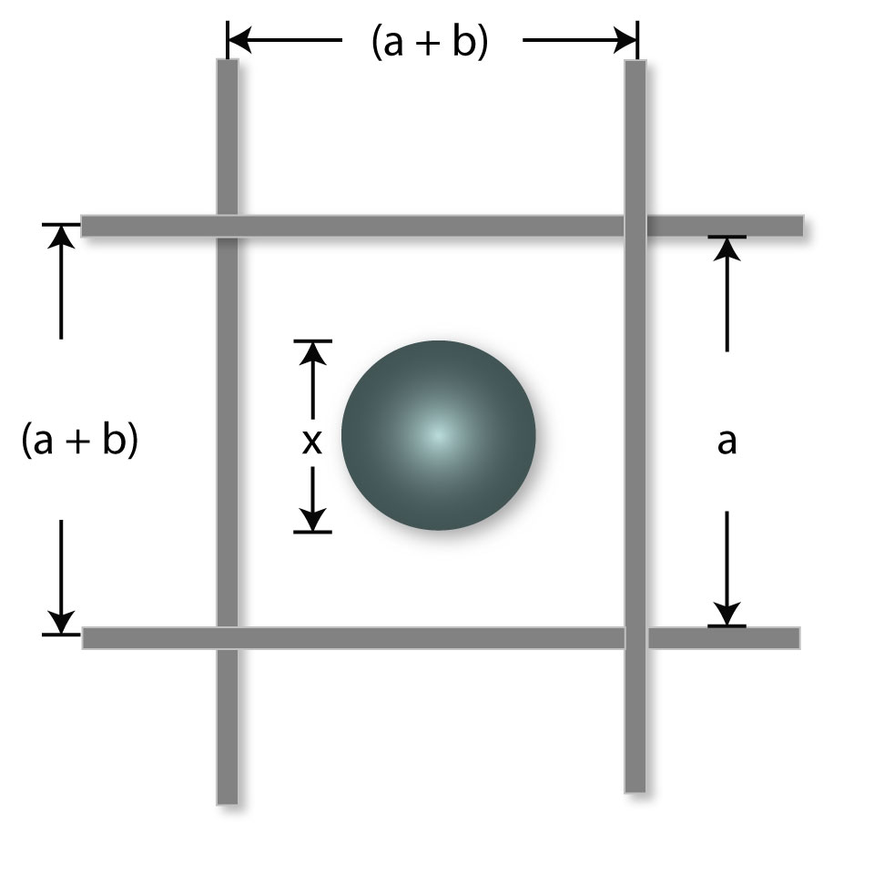
[image 145-1-4]
The probability of a particle being retained on a screen during a single trial Q is:
Q = 1-p [equation 4.2]
[equation 4.3]
m = number of screen trials which is a function of screen length, amplitude and frequency and assumes good stratification.
According to this simplistic model, the value of P increases with:
- Increasing screen opening a;
- Decreasing particle size x;
- Decreasing wire diameter b.
Screening Concepts
Also note that the probability P would increase over several trials m, and that m can be increased by increasing the length of the screen. Therefore, a perfect screening can only be achieved from an infinitely long screen.
However, the number of trials m possible on a given screen is a function of the amount of open area, As, available.
As – a2 / (a+b)2 = for square apertures
The amount of open area decreases significantly with a decrease in aperture size, e.g., 60% to 30%.
Screen manufacturers are using advanced materials and unique screen designs to increase open area.
[image 145-1-5]
![[image 145-1-5]](https://www.global.weir/assets/images/products/overview-images/TTH6203-V2_Image-05_Br141_CGI-P-WEB.png)
Percent Passing vs. Number of Trials
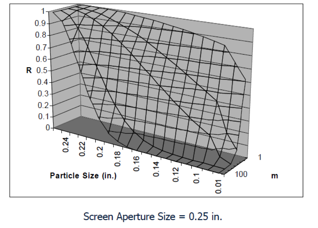
[image 145-1-6]
Perfect Screening vs. Reality
As mentioned previously, a 100% screening efficiency is not commercially practical since a screen of infinite length would be required.
A “perfect” separation is typically defined from a sieve analysis in which the sample is vibrated on a sieve for a period of 1 to 3 minutes. This is equivalent to approximately 90- to 180-feet long screen. A screen length of 24 feet is the largest manufactured screen.
The “commercial perfect” screening practice is typically based on efficiency values in the order of 90% to 95%, indicating that 5% to 10% of the undersize particles report to the screen overflow.
[image 145-1-7]
Screen Blinding Effects
Screen blinding reduces the number of openings in the screen, thereby decreasing the number of successful trials m.
Blinding is typically caused by particles having a 50% chance of passing through the screen. The critical particle size range that causes blinding is
0.5 < X/a < 1.5
Therefore, sizing of material having a large portion of material in the size class should be avoided.
High moisture and clay in the feed causes binding
[image 145-1-8]
![[image 145-1-8]](https://media.licdn.com/mpr/mpr/shrinknp_800_800/AAEAAQAAAAAAAAbBAAAAJDhkMDEyZDkzLTM3ZDMtNGYyZS05OTM3LTFmZmRlZWMzMThmZg.jpg)
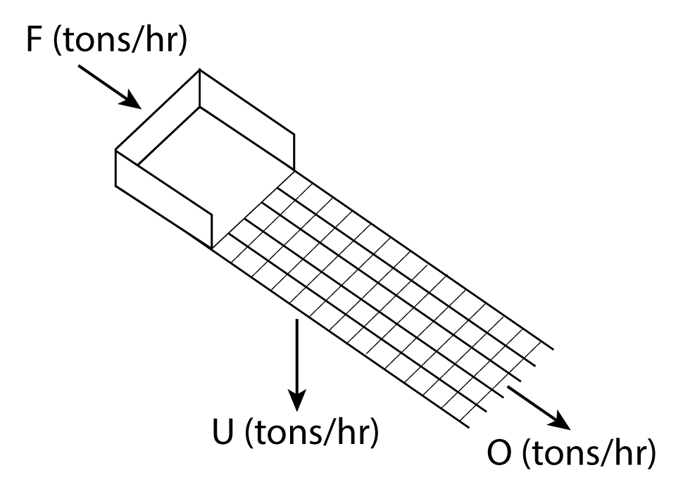
Mass Flow Rate Through a Screen
The mass flow rate at which particles flow through the screen varies as a function of distance from the feed point.
- From position a – b, the vibration of the screen causes the particles to stratify and the part1cle passage rate increases with distance .
- From position b – c, a maximum mass flow rate through the screen occurs and is referred to as “saturation screening”. This is due to the passage of the particles having a size significantly smaller than the aperture size.
From position c – d, the flow rate through the screen sharply declines since only those particles having a low probability remain.
[image 145-01-09]
Feed Rate vs. Efficiency
As previously mentioned, screens are designed to treat a given mass flow rate at which point a maximum screening efficiency value is obtained as shown below:
- At very low feed flow rates, screening efficiency increases with the feed rate. This is due to the fact that a sufficient amount of coarse particles is required to prevent excessive bouncing caused by screen vibration.
- At the point “a”, screening efficiency achieves an optimum value.
- Feed rates greater than the optimum value result in a decline in screening efficiency due to an increasing bed thickness and the inability of the undersize particles to report to the underflow stream, i.e., mass flow rate through the screen is limited.

[image (145-1.9)]
Screening Efficiency
Several definitions of screening efficiency exist, of which selected indexes are provided in the following sections.
Screening efficiency equation
Manufacturers express screening efficiency in terms of the content of undersize in the overflow b when the overflow is considered the product.
E = 100 – b [equation 4.4]
or
E = [% (or tph) of feed which is oversize/%(or tph) of feed which passes over] x 100
For example, assume a sieve analysis of the screen overflow revealed that 9% of the screen overflow is undersize material. According to the equation, the screen efficiency is 100 – 9 = 91%.
Two product formula - Oversize
Screening efficiency can also be determined by using the two product formula.
According to the two product formula, the recovery of oversize material to the screen overflow can be calculated using the following expression:
RO = OO / Ff = o(f-u) / f(o-u) [equation 4.5]
Where o, u, and f are the contents of the oversize material in the screen overflow, underflow and feed streams, respectively.
Two product formula - Undersize
Likewise, the corresponding recovery of undersize material to the screen underflow is:
Ru – (1-u) (o-f) / (1-f) (o-u) [equation 4.6]
Thus, the overall screening efficiency E is the product of Ro and Ru or:
E = 0(f-u) / f(o-u)2 x(1-u) (o-f) / (1-f) [equation 4.7]
It should be noted that if no apertures are deformed or broken, then the concentration of oversize in the underflow stream is approximately zero and, thus, Eq. [4.7] reduces to Eq. [4-6]:
Performance Prediction & Efficiency Assessment
Partition curves are also commonly used to determine the separation efficiency whereby the Imperfection Value ” ” can be obtained:
I = d75 – d25 / 2d50 [equation 4.8]
where the d75, d50, and d25 are the particle sizes that have a 75%, 50%, and 25% chance of reporting to the overflow stream.
Partition curves from a screening process are most useful for predicting the outcome for each size fraction comprising the feed. Thus, an overall knowledge of the overflow and underflow stream compositions can be obtained.
[image 145.1.11]
[image 145-1-12]
Prediction Screen Performance
Whiten and White (1997) defined a partition curve model for single deck screens based on screen open area (fa) and an efficiency parameter (TRN) that is a function of the number of trial events on the screen, i.e.,
Y(x) – exp[ -TRN (fo) (1 – x / d)2] [equation 4.9] where Y is the actual partition number in terms of the probability to the overflow stream, TRN the efficiency parameter, fa the fractional open area, and d the screen aperture size.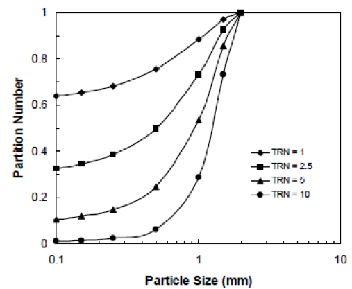
- TRN is a function of feed rate and the decking material. For rubber decking, an optimum feed rate exists.
- Fractional open area has the same effect on screening efficiency as the TRN value.
An inclined screen deck with a 2 mm aperture is being used to achieve a size separation for a given material. Assume a TRN value of 10 and no ultra-fine particle agglomeration or sliming, predict the particle size distribution of the overflow and underflow streams given the following feed size distribution.
Predict the Particle Size Distribution Given:
| Particle Size Fraction (mm) | Weight (tph) |
|---|---|
| +2 | 30 |
| 2 x 1 | 25 |
| 1 x 0.6 | 20 |
| 0.6 x 0.3 | 10 |
| 0.3 x 0.15 | 5 |
| -0.15 | 10 |
Distribution Solutions
| 1 | 2 | 3-1*2 | 4=1-3 | |||
|---|---|---|---|---|---|---|
| Particle Size (mm) | Feed Weight (ton.hr) | Partition # (Eq. 10) | Overflow (tph) | Overflow (%) | Underflow (tph) | Underflow (%) |
| +2 | 30 | 1.000 | 30.00 | 60.04 | 0.00 | 0.00 |
| 2 x 1 | 25 | 0.651 | 16.28 | 32.58 | 8.72 | 17.43 |
| 1 x 0.6 | 20 | 0.153 | 3.06 | 6.13 | 16.94 | 33.85 |
| 0.6 x 0.3 | 10 | 0.045 | 0.45 | 0.90 | 9.55 | 19.09 |
| 0.3 x 0.15 | 5 | 0.018 | 0.09 | 0.18 | 4.91 | 9.81 |
| -0.15 | 10 | 0.008 | 0.08 | 0.16 | 9.92 | 19.82 |
| 100 | 49.96 | 100.00 | 50.04 | 100.00 |
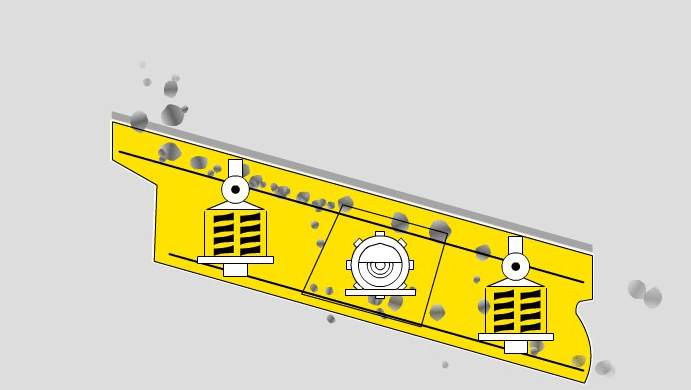
Screen Selection
Screen selection is based on the overall screen area required to achieve efficient screening at a given mass throughput capacity .
- Length of screen is important for ensuring the number of trials needed to achieve the desired mass throughput capacity and to provide sufficient screen underflow capacity.
- Width is important for ensuring proper bed depth so as to provide sufficient stratification.
- Length of screen should be at least two times the width for good practical design.
Screen Area
The required screen area A can be determined by the expression:
A = Fu / TC [equation 4.10]
F = the feed rate in tons per hour,
u = the percentage of material in the feed liner than the screen opening,
T = screen capacity in terms of the throughput (tons/hour) passing through the screen per linear foot;
C = represents correction factors for the screen capacity based on variations from the standard (or default) parameter values, i.e,
= C1 x C2 x C3 x C4 x C5 x C6 x C7 x C8 x C9 x C10 x C11 [equation 4.11]
The value for u can be obtained from the cumulative percent finer curve representing the particle size distribution of the screen feed.
Correction Factors
| Corrections | Definitions |
|---|---|
| C1 | Mass factor |
| C2 | Open area factor |
| C3 | % Oversize material in feed |
| C4 | % Undersize (fines) in feed |
| C5 | Screen efficiency factor |
| C6 | Deck factor |
| C7 | Screen factor |
| C8 | Adjustment to aperture shape |
| C9 | Adjustment to particle shape |
| C10 | Adjustment to wet screening |
| C11 | Adjustment due to moisture |
Screen Capacity, T
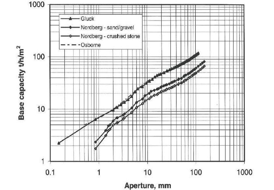
[image 145-1-14]
Gluck assumes bulk density= 1.6 t/m3
Nordberg (Metso): 50% oversize in feed, size, 25% half size, 20 ° slope, 92%-95% efficiency.
Osborne: 60 °/o open area.
Mass Correction Factor, C1
Standard factors were developed using normal vibrating speeds using a material having a density of 1.602 t/m3.
Where the solid density is different, the following correction is applied:
C1 = Ï / 1.602
Open Area Correction Factor, C2
Corrects for percentage of available open area.
The standard percentage of open area for a given aperture size is provided by the manufacturer capacity plot.
C2 = Pa / Pr [equation 4-12]
Pa = actual % open area,
Pr = rated % open area obtained from plot
Pa = 100 A1 A2 / (A1 + W1) (A2 + W2) for rectangular openings
[equation 4-13]
Pa = 100 A2 / (A + W)2 for square openings [equation 4-14]
Pa = 100 A / (A + W) for wedge wire [equation 4-15]
A = aperture or screen opening
W = wire or bar diameter
Base Open Area vs. Screen Aperture

[image 145-1-15]
Correction Factor for Oversize, C3
25% oversize is the standard and any different value affects the stratification process
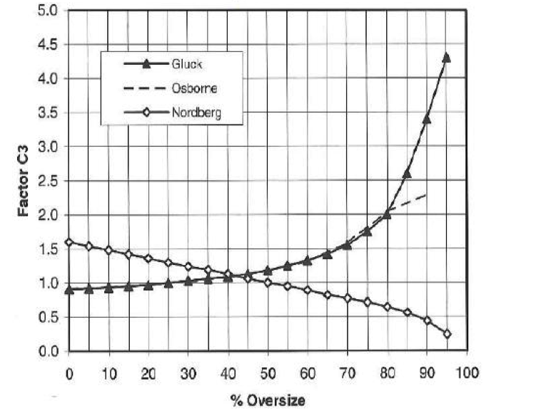
[image 145-1-16]
Correction for Undersize, C4
Defined as the percent less than half the screen aperture and the standard is 40%.
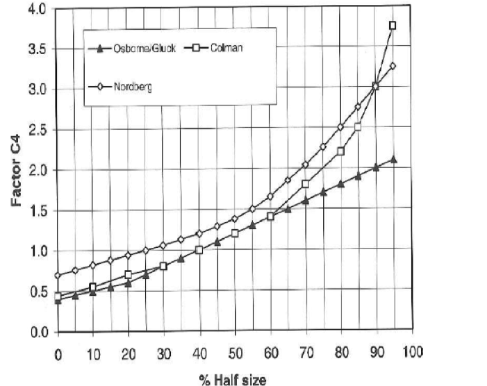
[image 145-1-17]
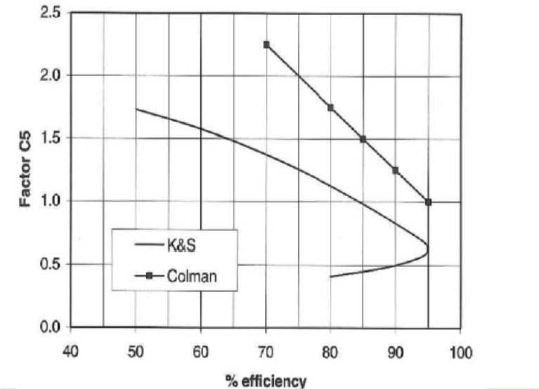
Screen Efficiency Factor, C5
90% – 95% is considered normal for a typical woven wire screen. Colman recommends 80% – 85% for scalping operations.
[image 145-1-18]
Multi-deck Correction Factor, C6
This factor accounts for the fact that lower decks have an effectively lower screen surface area since the majority of the material from the top deck enters the next further down the screen.
It is applied to the design of each deck below the top deck.
For a n number of decks from the top, the correction factor is:
C6 = 0.9(n-1) [equation 4-16]
[image 145-1-19]
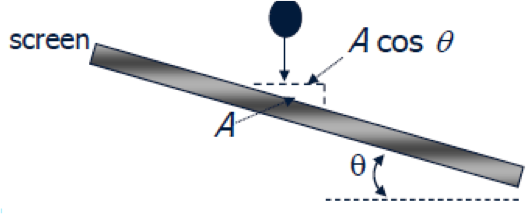
Screen Slope Correction, C7
Corrects for the reduction in effective horizontal screen area:
[image 145-1-20]
Ahorizontal = A cos θ [equation 4-17]
A = aperture length along the slope
θ – angle of inclination from horizontal
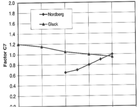
[image 145-1-21]
Correction for Aperture Slot Shape, C8
| Aperture Shape | Gluck | Colman | Nordberg | |||
|---|---|---|---|---|---|---|
| L/W | C8 | L/W | C8 | L/W | C8 | |
| Square | 1 | 1 | <2 | 1 | 1 | 1 |
| Rectangle | >6 | 1.6 | >25 | 1.4 | 3-4 | 1.15 |
| Rectangle | 3-6 | 1.4 | 4-25 | 1.2 | >4 | 1.2 |
| Rectangle | 2-3 | 1.1 | 2-4 | 1.1 | ||
| Circular | -- | 0.8 | -- | 0.8 | ||
Correction for Particle Shape, C9
Elongated particles are defined as a particle having a length-to-width ratio greater than 3 and a size between 0.5 and 1.5 times the aperture size.
![Charting correction for particle shape C9 [image 145-1-22]](https://millops.community.uaf.edu/wp-content/uploads/sites/605/2016/10/145-1-22-chartingCorrectionforParticleShapeC9.png)
[image 145-1-22]
Correction for Wet Screening, C10
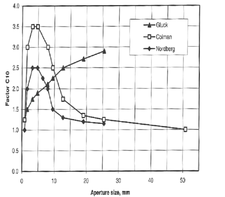
[image 145-1-23]
Correction for Moisture, C11
| Condition | C11 |
|---|---|
| Moist or dirty stone, muddy or sticky | 0.75 |
| Moist ore from underground, >14% moisture | 0.85 |
| Dry quarried rock <4% -10% | 1.00 |
| Dry uncrushed material, dry or hot material | 1.25 |
| Wet screening with sprays | 1.75 |
Typical Commercial Screens
| Width (mm) | Area (m2) | | | Width (mm) | Area (m2) | | | Width (mm) | Area (m2) |
|---|---|---|---|---|---|---|---|
| 254 | 0.31 | | | 1524 | 5.57 | | | 2134 | 10.41 |
| 305 | 0.37 | | | 1219 | 5.95 | | | 1829 | 11.15 |
| 356 | 0.43 | | | 1524 | 6.50 | | | 2134 | 11.71 |
| 356 | 0.54 | | | 1829 | 6.69 | | | 2438 | 11.89 |
| 610 | 0.56 | | | 1524 | 7.43 | | | 2134 | 13.01 |
| 406 | 0.62 | | | 1829 | 7.80 | | | 2438 | 13.38 |
| 610 | 0.74 | | | 1524 | 8.36 | | | 2438 | 14.86 |
| 406 | 0.74 | | | 1829 | 8.92 | | | 2438 | 17.84 |
| 508 | 0.93 | | | 2134 | 9.10 | | | ||
| 508 | 1.08 | | | 1524 | 9.29 | | | ||
| 610 | 1.11 | | | 1829 | 10.03 | | |
The depth of the bed at the discharge end of the screen indicated the effectiveness of the bed stratification and the ability of particles to have an opportunity to pass through the screen.
The bed depth, D, in inches at the discharge end should be limited to limit to 4 times the screening opening for solid density > 100lbs/ft3 or 3 times for less than 100lbs/ft3.
The expression used to quantify D is:
D = TK/5SW [equation 4-18]
T = tons/hour at discharge end.
K = cubic feet per ton of ore; or 2000lbs/ton divided by the solid density in lbs/ft3.
S = material travel rate in feet per minutes which is dependent on screen and material characteristics.
- Horizontal screens have travel rates of about 45 feet/minute.
- Incline screens having a 20 ° slope have travel rates of about 125ft/min. A reduction in slope reduces the screen capacity as shown in the following table.
W = net width of the selected screen in feet. Due to support material the net width = nominal width – 6 inches.
Screens Width Design
| Slope Reduction | % of Rated Capacity |
|---|---|
| 2-1/2 degrees or less | 90 - 92.5 |
| 5 degrees or less | 80 - 85 |
| 7 - 1/2 degrees or less | 70 - 75 |
| 10 degrees or less | 60 - 65 |
If the selected width provides a bed thickness greater than the maximum allowable, then
- Choose a wider screen (less length);
- Choose a larger screen area;
- Increase the screen inclination (increase S );
- Use multiple decks (the use of an upper deck to remove a coarser size fraction will unload the final sizing deck).
Then, repeat the bed depth calculation.
Screens Width Design (Metric units)
The expression used to quantify D (mm) is:
D = 50T/3SWK [equation 4-19]
T = metric tons of overflow material
K = bulk density of material (tjm3)
S = material travel rate in meters per minute which is dependent on screen and material characteristics.
W = effective width of screen (m). Due to support material in the net width = nominal width – 0.15.
For material of bulk density 1.6 t/m3, the bed at the feed end should not exceed 4 times the aperture size.
For material of bulk density 0.8 t/m3, the bed depth should not be greater than 2.5 – 3.0 times the aperture size.
Screens Design Considerations
For screen widths of 0.6 – 2.5 meters, the inclination should not be less than 16 ° and a maximum of about 26 ° for capacities 15 – 270 t/h.
When the slope is greater than 20 degrees, the capacity is markedly reduced as the effective aperture area is reduced by 0.93.
For longer screens, e.g. 4.8 meters, screen manufacturers recommend a further addition of 2 degrees and for screens of about 6 meters, 4 degrees should be added.
Adequate Screens Length Assessment
A function of the undersize materials ability to screen within a given period of time.
Sufficient length is needed to provide sufficient residence time to maintain desired screening efficiency.
The appropriate residence time can be determined by analyzing the screening efficiency as a function of time using a standard lab sieve shaker and the exact screen aperture that is or will be used in the plant.
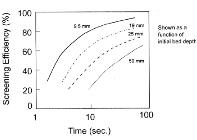
[image 145-1-24]
A processing engineer is assigned the task of determining the screen area required to screen 200 tons/hr of minerals at a 3/4-inch particle size. The material density is 150 lb/ft3 and the Rosin/Rammler constants are R=0.5 inches and =0.8. The screen should have square openings with 5/16″ wires. Water sprays will be used. Assume an oversize velocity of 1 ft/sec.
Solution:
A = FU/TK
F = 200tph
T = ?? from graph
Underflow (%) -> Rosin-Rammler Eq.
Y = 1 – exp[-(x/R)n]
U = Y = 1 – exp[ -(0.75/0.5)0.8] = 0.749 = 0.75
K = KaKoKuKwKdKs
- Open Correction Factor, Ka
Ka = Pa/Pr
Pa = 100A2 / (A + W)2 = 100 (3/4)2 / (3/4 + 5/16)2 = 49.83
From graph:
Pr = 56%
Ka = 49.8/56 = 0.889 - Oversize Correction, Ko = 1.0 from graph
- Undersize Correction, Ku = 1.3 from graph
Y = 1 – exp [-(0.375/0.5)0.8] = 54.8 - Wet Screen Correction, Kw – 1.1 from table
- Safety Correction, Ks – 0.8
- Kd = 1
K = (0.889) (1.0) (1.3) (1.1) (0.8) = 1.017
A = (200 tph) (0.75) / (??? tph/ft2) (1.017) = 83.8 ft2
Assume 16′ x 6′ screen:
D = TK/5SW = 200 tons/hr * 0.25 * ???ft3 /ton / 5*60ft/min * 6 ft = 0.925
Since 0.93″ < (3 x 3/4″) the chosen screen is acceptable
With 10% support:
Area = 83.8 x 1.1 = 96ft2
Save