Contents
Reading
Classifying cyclones are the most commonly used technology for achieving particle size separations below 300 microns.
Classifying cyclones are comprised of a cylindrical section and a conical section. The length of the conical section has been found to significantly effect particle size separations
Cyclone Fundamentals
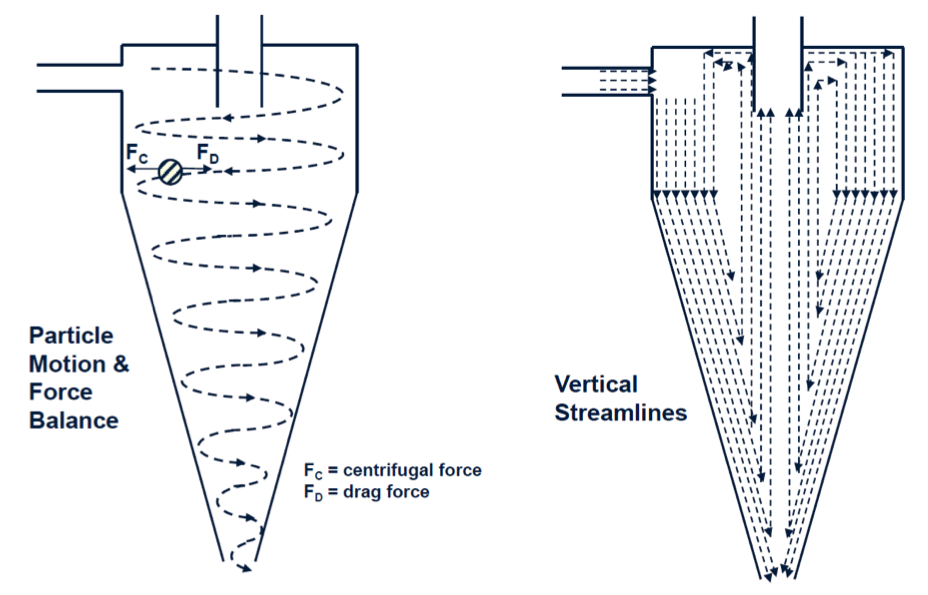
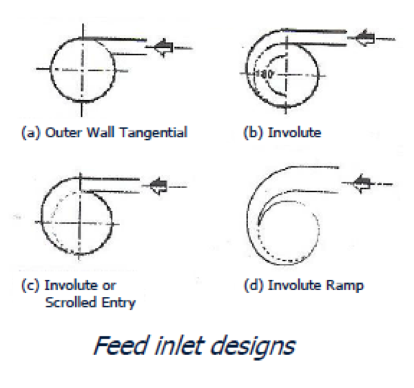
A tangential feed injection is used to induce a centrifugal force, which accelerates the particle size settling kinetics.
Coarse particles report to the outer wall of the cyclone and spiral downward toward the apex or spigot via the motion of the fluid stream.
Due to a constricted apex, the volume reporting to the underflow stream is restricted and thus a portion of the stream is forced to reverse direction and move upward along a low pressure zone toward the Vortex Finder. The upward moving flow carries the fine particles to the overflow stream.
[image 145-2-1]
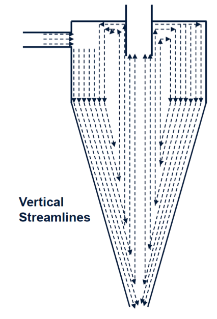
Radical & Vertical Flow Profiles
[image 145-2-2]
Design
The magnitude of the applied centrifugal force increases with a decrease in cyclone diameter. As such, the cyclone diameter selected for a given application is associated with the desired size separation.
In mineral applications. it is generally stated that a certain size cut is desired which would imply that the majority (i.e., 95%) of underflow solids has a size greater than the target cut point and the overflow has a majority less than the desired cut point.
However, design models are based on the particle size that has a 50% probability of reporting to the overflow or underflow stream.
It is generally recognized the small particle size separations require small diameter hydrocyclones. For geometrically equivalent cyclones, the mean particle size separation (d50) is a function of the cyclone diameter, i.e.,
d50(c) = DCX
where the value of x has been debatable and vary from model to model as shown below:
- 1.875 → Krebs-Mular-Jull Model (1978);
- 1.8 → Plitt’s Model (1976);
- 1.36 to 1.52 → Bradley’s Model (1965).
D50(c) Versus Overflow Size Relationship
A relationship between the d50(c) and the overflow size was developed by Arterbury (1976).
For example, it is typically desired to achieve a 100 mesh (150 micron) separation.
- 95% -100 mesh in overflow.
- Multiplier = 0.73.
- Target d50(c) = 150 x0.73 = 110 microns
| Required Overflow Size (% passing) | Multiplier |
|---|---|
| 98.8 | 0.54 |
| 95.0 | 0.73 |
| 90.0 | 0.91 |
| 80.0 | 1.25 |
| 70.0 | 1.67 |
| 60.0 | 2.08 |
| 50.0 | 2.78 |
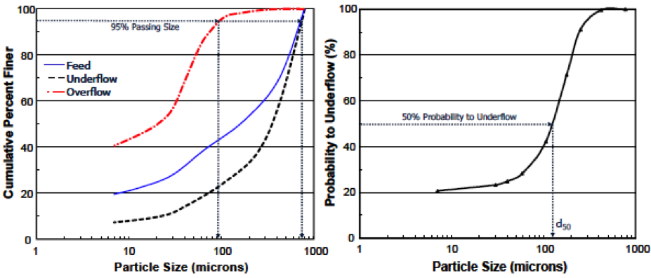
d50 Versus 95% Finer
[image 145-2-3]
- Particle size distributions of the feed, underflow and overflow streams.
- d95 (overflow) = 95 microns.
- d95 (underflow & feed) = 750
- Due to inefficiencies, every particle in the feed has a probability of reporting to either the underflow or overflow streams.
- The particle size having a 50% chance of reporting to either stream is the d50.
Plitt Equation
A commonly used design model used for applications in the mineral industry was design by Plitt (1976), i.e.,
in which d50(c) is in microns, Q in m3/hour, Dc , Di , Du and Do the cyclone cylinder, inlet, spigot and vortex finder diameters in centimeters, h the distance in cm from the bottom of the vortex finder to the top of the apex, P the feed pressure in kPa (1 psi = 6.895 kPa), Ïs the density of solids in grams/cm3, and V the volumetric percent solids concentration in the feed.
The definition of a ‘typical’ cyclone is:
- Inlet area ≈7% of the cross-sectional area of the cylindrical chamber.
- Vortex Finder diameter = 30% of the cyclone diameter.
- Apex diameter = 10%-35% of the cyclone diameter.
- Cone Angle = 10 ° – 20 °
Classifying Cyclone Design (Krebs Engineers)
Krebs Engineers approach cyclone design similar to screen design.
Cyclone design is based on the d50(c) achieved using a typical cyclone under standardize conditions, i.e.,
- Medium = water at 20 °C & 1 centipoise
- Solids density= 2.65
- Solids concentration < 1%.
- Pressure drop = 10 psi.
The base d50(c) can be estimated by the expression:
d50(c) (base)=2.84DC0.66
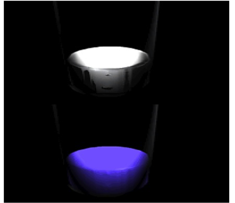
Viscosity
[image 145-2-4]
Krebs Cyclone Design
The actual d50(C) can be determined from the expression:
d50(c) (actual) = D50(c) (base) x π1m CPm x π1n CDn
in which CPm are the correction factors for m process variables and CPn the design related factors.
Process variable include feed solids content, solids density, pressure drop and slurry viscosity.
Cyclone design parameters include cyclone diameter, vortex finder diameter, spigot diameter, length of cylinder, cyclone, cyclone angle and mounting angle.
![Cyclone design graph [image 145-2-5]](https://millops.community.uaf.edu/wp-content/uploads/sites/605/2016/10/145-2-5-cyclonedesigngraph.png)
[image 145-2-5]
Feed Particle Size & Solids Content Correction
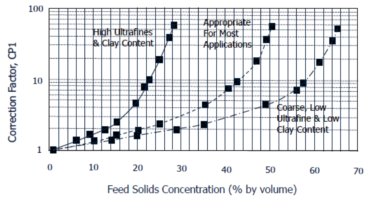
[image 145-2-6]
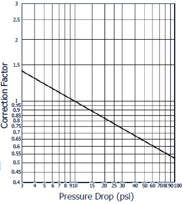
Pressure Drop Correction
Pressure drop within a given operation can be adjusted through a change in volumetric feed rate.
- Variable feed pumps.
- Valves on feed lines which opens or closes the flow to cyclones in a bank.
A change in feed pressure has a relatively small effect on the d50(c).
The expression for the determination of the correction factor is:
CP(pressure) = 3.27p-0.28
Where P is the pressure drop in kPa
[image 145-2-7]
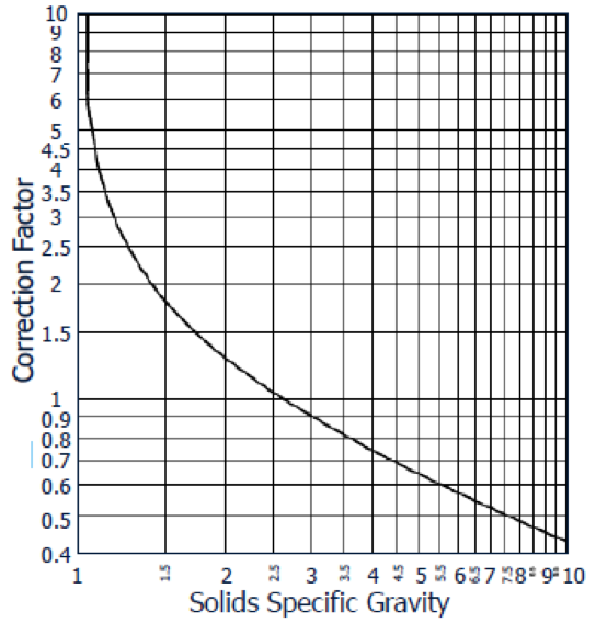
Solid Density Correction
The rate that a charged particle moves in a fluid under centrifugal forge is a function of particle density.
Higher density particles move at a faster rate toward the cyclone wall. As such, the d50(c) for high density particles is lower.
The correction factor for solid density is:
CP(density) = [1.65/(Ïs-Ïm)]-0.5
Where Ïs and Ïm are the densities of the solid and medium in gm/cm3.
[image 145-2-8]
Cyclone Design Corrections
Inlet Diameter
- Effects both feed flow rate capacity and d50(c).
- Manufacturers can provide different sizes and shapes to meet flow rate capacities.
- In general, an increase in inlet size elevates capacity and the d50(c).
Cylinder Length
- Increasing length results in greater retention time which should reduce d50(c).
- Typically, the cylinder length is equal to the cyclone diameter.
Large cyclones (>660 mm) use shorter cylinder lengths.
[image 145-2-9]
Cone Section
Cone angles vary from 6 ° to 90 °
20 ° cone angle has been the standard; however, 10 ° is common for cyclones in the mineral industry
High cone angles are typically used to achieve very coarse particle size separations
Longer 10 ° cones achieve higher retention times and finer, more efficient size separations.
Recently, Krebs Engineers developed the qMax cyclone which incorporates a dual slope cone, i.e., a 10 ° at the interface between the cylinder and the cone and a 6 ° angle at the bottom of the cone. Retrofitting a standard cyclone allows lower d50(c).
Vortex Finder
- Primary role is to control the size separation and the flow leaving the cyclone.
- Extended below the inlet to prevent feed bypass
- Size can range from 20% – 45% of the cyclone diameter
- Large vortex finders increase capacity and elevates the d50(c)
- The expression to determine the correction factor is:
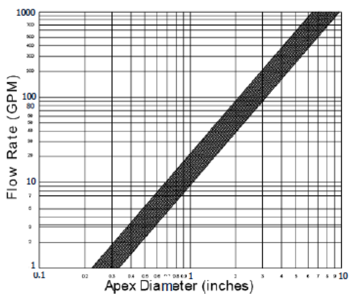
Apex Diameter
- Must be large enough to allow passage of the expected amount of flow.
- Has some effect on the d50(c).
- Correct size is typically selected after the cyclone size and number has been determined and a material balance has been performed.
- The pattern of the discharge is indicative of performance: a) a wide angle indicates unacceptable solids content and ‘roping’ conditions represent excessive solids content and poor performance
[image 145-2-10]
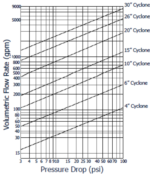
Volumetric Feed Flow Rate
The volumetric feed rate to a cyclone is directly related to the pressure drop across the cyclone.
As such, the pressure drop used for determining the d50(c) is applied to determine the feed flow rate per cyclone.
To determine the number of cyclones needed, the total flow rate of the stream is divided by the allowable flow rate per cyclone (see attached graph).
The data shown in the graph was obtained using water. Therefore, the determination of the number of cyclones will be a slight over estimation.
[image 145-2-11]
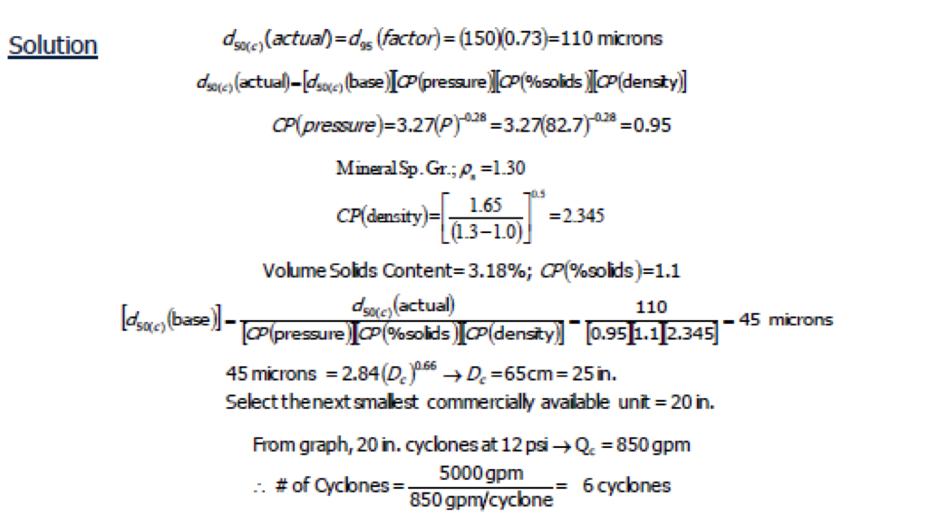
Design Example
A classifying cyclone system is needed to achieve a 150 micron (100 mesh) separation. The total volumetric flow rate to the system is 5000 gpm at a solids content of 5% by weight (Ïp=1.02). At an average relative solids density of 1.3, the solids mass flow rate equates to 64 tons/hr. The desired operating pressure is 12 psi (82.7 kPa). A standard vortex finder size will be used.
[image 145-2-12]
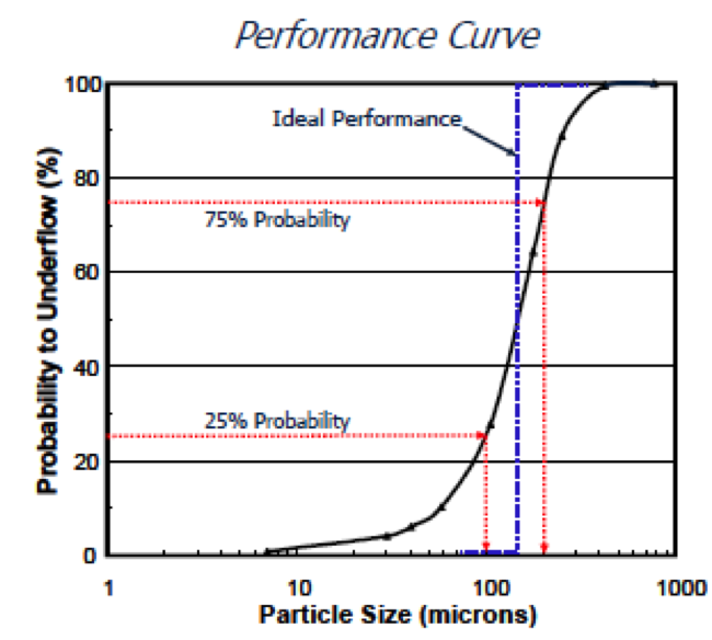
Performance Prediction
The efficiency of a classifying cyclone is typically measured by the slope of the partition curve plotted on the basis of the probability of a particle reporting to the underflow stream versus particle size.
A more direct efficiency measurement from the partition curve is the imperfection value (I):
I = d75 – d25 / 2d50
in which d75, d50, and d25 are the particle sizes having 75%, 50%, and 25% probabilities, respectively, of reporting to the underflow stream
[image 145-2-13]
Example: Partition Curve Development
The mass yield of solids to the underflow has been determined to be 63% using the two-product formula. A particle size analyses of samples collected from the underflow and overflow streams have been completed and the results provided:
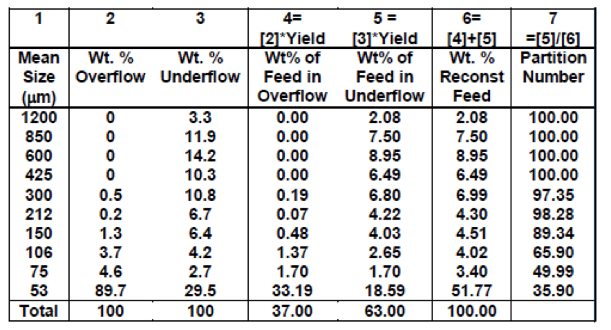
[image 145-2-14]
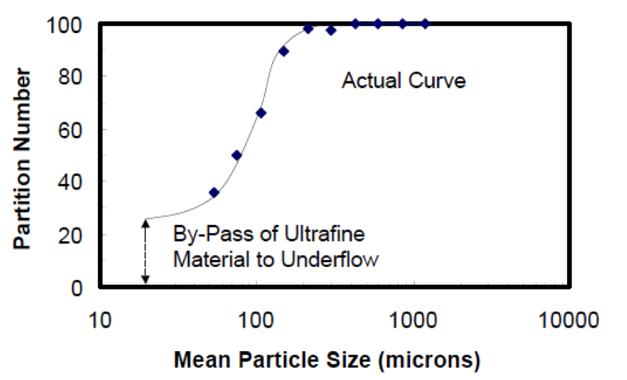
Actual Partition Curve
A plot of Column [7] versus Column [1] forms the Actual Partition Curve which is shown in the following figure.
[image 145-2-15]
Ultrafine By-Pass
An inherent inefficiency of classifying cyclones is that the water recovered in the coarse underflow stream carries ultrafine particles that should be in the overflow stream. The by-pass is typically referred as ultrafine by-pass.
From the figure in the previous slide, the amount of ultrafine by-pass is indicated by the probability corresponding to the smallest size fraction, which is around 26%.
In general, an increase in water recovery results in an increase in the amount of ultrafine by-pass.
A worn apex will result in an increase in water recovery and thus increase ultrafine by-pass.
In design, it is commonly desired to minimize the apex size to limit water recovery. Solid concentrations as high as 50% by weight can be achieved without roping conditions.
Since ultrafine by-pass is not related to the actual separation of particles based on the applied forces within the cyclone, the effect of ultrafine by- pass on the Actual Partition curve is removed before measuring the true efficiency by the Imperfection value (Eq. 10-9).
The correction for ultrafine by-pass results in the Corrected Partition Curve.
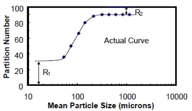
Correction Partition Curve
The equation for determining the corrected Partition Number is:
In which Y’ is the corrected partition number, U the actual partition number, R1 the fractional amount of ultrafines by-passing to the underflow stream and R2 the fractional amount of coarse particles by-passing to the overflow stream.
The by-pass of coarse material to the overflow stream is rare but may occur due to a worn vortex finder.
R2 = 0 can be assumed in most cases.
[image 145-2-16]
Example
Based on the curve projection, the estimated amount of ultrafine by-pass in the example was about 26%.
Using the equation above, the corrected partition number for each size fraction can be determined.
| 1 | 2 | 3 |
|---|---|---|
| Mean Particle Size (microns) | Actual Partition Number | Corrected Partition Number |
| 1200 | 100.00 | 100.00 |
| 850 | 100.00 | 100.00 |
| 600 | 100.00 | 100.00 |
| 425 | 100.00 | 100.00 |
| 300 | 97.35 | 96.42 |
| 212 | 98.28 | 97.68 |
| 150 | 89.34 | 85.59 |
| 106 | 65.90 | 53.92 |
| 75 | 49.99 | 32.42 |
| 53 | 35.90 | 13.38 |
Corrected Partition Curve
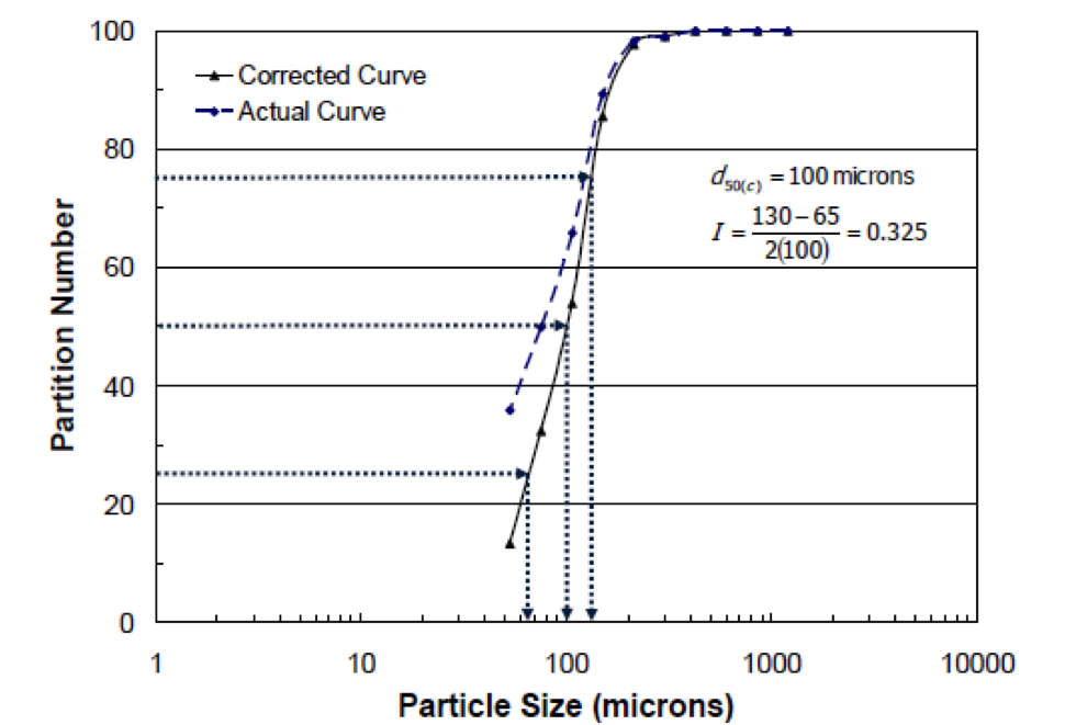
[image 145-2-17]
Reduced Efficiency Curves
Lynch and Rao (1965) found that classifying cyclone efficiencies are more easily evaluated and compared over a range of cyclone geometries and operating conditions using a Reduced Efficiency Curve.
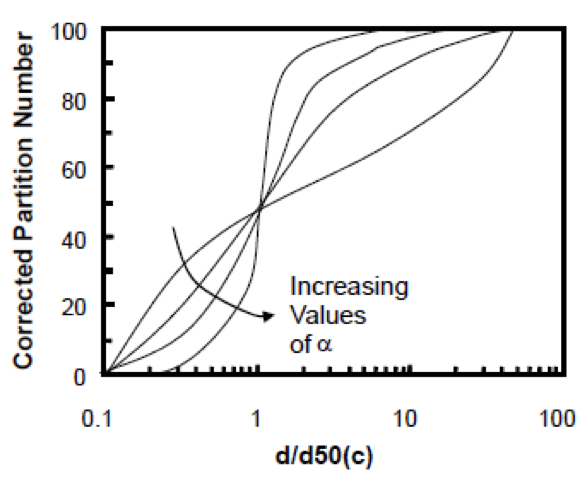
The Reduce Efficiency curve is a plot of the corrected partition numbers versus (d/d50(c)).
Separation Performance Projection
Lynch and Rao found that the Reduced Efficiency Curve can be modeled by the following expression:
in which x is the d/d50(c) and a is the curve slope and the value is indicative of the classification efficiency.
Typical α values are between 2 and 4.
The equation above can be used to predict the performance of a classifying cyclone by assuming a value for α.
[image 145-2-18]
Example: Performance Prediction
Given a feed particle size distribution and an alpha value of 2.5, predict the performance of a cyclone. The amount of ultrafine by-pass is assumed to be 20% by weight.
| 1 | 2 | 3 | 4 | 5 | 6 = 2*5 | 7= 6/(Σ6) |
|---|---|---|---|---|---|---|
| Mean Particle Size (microns) | Weight (%) | d/d50(c) | Corrected Partition Number | Actual Partition Number | Underflow Weight (%) | Normalized Underflow Weight (%) |
| 1200 | 2.40 | 12 | 1.00 | 1.00 | 2.40 | 3.90 |
| 850 | 7.50 | 8.5 | 1.00 | 1.00 | 7.50 | 12.18 |
| 600 | 8.90 | 6 | 1.00 | 1.00 | 8.90 | 14.45 |
| 425 | 6.40 | 4.25 | 1.00 | 1.00 | 6.40 | 10.39 |
| 300 | 6.90 | 3 | 1.00 | 1.00 | 6.89 | 11.19 |
| 212 | 4.30 | 2.12 | 0.97 | 0.97 | 4.19 | 6.80 |
| 150 | 4.50 | 1.5 | 0.82 | 0.86 | 3.86 | 6.28 |
| 106 | 4.00 | 1.06 | 0.55 | 0.64 | 2.55 | 4.14 |
| 75 | 3.40 | 0.75 | 0.31 | 0.45 | 1.52 | 2.46 |
| 53 | 51.70 | 0.53 | 0.17 | 0.34 | 17.36 | 28.20 |
| Total | 100.00 | 61.57 | 100.00 |
Feed
- Qf = 5000 gpm; Mf = 64 tph
Underflow
- Solids Yield to Underflow = 61.57%
- Mu = 64 tph (0.6157) = 39.4 tph
- Assume a desired underflow solids content of 40%
- Total Mass Flow = 39.4/0.40 = 98.5 tph
- Calculated Pulp Density = 1.176 (based on Ïp = 1.6)
- Qu = 335 gpm → 335 gpm/6 = 56 gpm/cyclone
- Apex Diameter → 2 inches (from graph)
Overflow
- Mo = 24.6 tph
- Qo = 4665 gpm → 778 gpm/cyclone
Transporting the slurry into and out of the cyclone circuit requires a line velocity of 7 — 10 ft/sec (200 — 300 cm/sec) to keep particles suspended.
Feed enters a center chamber for distribution where the slurry velocity should be reduced to 2 — 3 ft/sec (60 — 90 cm/sec) to ensure good distribution.